Principal-Component-Analysis
First introductions to Principal component analysis are usually delivered via so-called maximum variance or minimum reprojection error formulations, both of with lead to eigenvalue problems. Another useful view is that of probabilistic PCA, which is the subject of this post. The probabilistic view offers a number of benefits and generalisations. Two useful sources of information are chapter 12.2 of Bishop’s book and chapter 10.7 of Mathematics for Machine Learning.
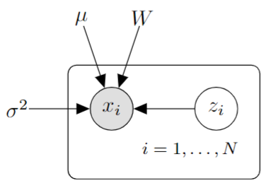
A Graphical model
We are given access to a dataset \(X \in \mathbb{R}^{N \times d}\), which represents \(N\) vectors \(x_i \in \mathbb{R}^d, \quad 1 \leq i \leq N\). Let \(l < d\). We assume that the observed data are samples from a conditionally multivariate Gaussian distribution given some latent variables \(Z \in \mathbb{R}^{N \times l}\), representing \(N\) vectors \(z_i \in \mathbb{R}^l, \quad 1 \leq i \leq N\). The expected value of the Gaussian is \(Z W^\top + 1_{N \times 1} \mu^\top\) for some deterministic parameters \(W \in \mathbb{R}^{d \times l}\) and \(\mu \in \mathbb{R}^{d}\). The covariance matrix of the Gaussian is diagonal with deterministic entry \(\sigma^2\). The distribution over \(Z\) is an uncorrelated standard Gaussian. This leads to the graphical representation as shown.
Parameter estimation and inference
Given our model, we may estimate the values of \(W\) and \(\mu\) by maximum likelihood estimation, and infer the distribution over \(Z\) by examining the posterior. Since the Gaussian distribution is in some sense closed under marginalisation and conditioning, the marginal likelihood and posterior can be found in closed form. These are
\[p(X \mid W, \mu, \sigma^2 ) = \prod_{i=1}^N p(x_i \mid W, \mu, \sigma^2 ), \quad p(x_i \mid W, \mu, \sigma^2 ) = \mathcal{N} (\mu, W W^\top + \sigma^2 I )\]and
\[p(z_i \mid x_i, W, \mu, \sigma^2) = \mathcal{N}(m, C), \\ m = W^\top(W W^\top + \sigma^2 I)^{-1}(x_i - \mu), \\ C = I - W^\top(W W^\top + \sigma^2 I)^{-1} W.\]Maximum likelihood estimates can be computed in closed-form or numerically, both with their own advantages and caveats. See Bishop for details.
Why the probabilistic view can be useful
The probabilistic view can be used as a starting point for various generalisations of PCA. Bayesian PCA treats parameters \(W\), \(\mu\) and \(\sigma^2\) as random variables. Exponential family PCA replaces the Gaussian likelihood with an exponential family likelihood. Bayesian exponential family PCA mixes these ideas. When there is a large amount of data, computing the reduced eigendecomposition of the covariance matrix can be challenging. Numerical optimisation of the likelihood can assist in this computation, as can the EM algorithm.